4 Extremes of Non-identically Distributed Variables

Though it is possible to study the asymptotics of maxima of processes with specified forms of non-identically distributed variables, the results are generally too specific to be of use in modelling data for which the form of departure from identically distributed is unknown.

Since many interesting data sets are in fact non-identically distributed the question of how to produce good models in this situation is an interesting and important one. We begin by examining some examples of non-identically distributed processes. We shall then discuss some of the existing ideas on how to model such processes, before introducing an alternative approach which allows us to use information in the entire process to define the extremes.

4.1 Examples of non-identically distributed processes

We look at two examples of non-identically distributed processes;

Simulated data - where we can specify different kinds of marginal distribution;
Reading ozone data set.

We shall discuss what it means for a process to have non-identically distributed margins and some of the forms that this may take. These forms of non-identical distribution are specifically chosen to lead into the modelling approach discussed in Section .

Trend in mean level
The simplest form of non-identical marginal distribution is to have a trend in the mean (average) of a process. Here we show linear and cyclic (or seasonal) trends in Figure 4.1.

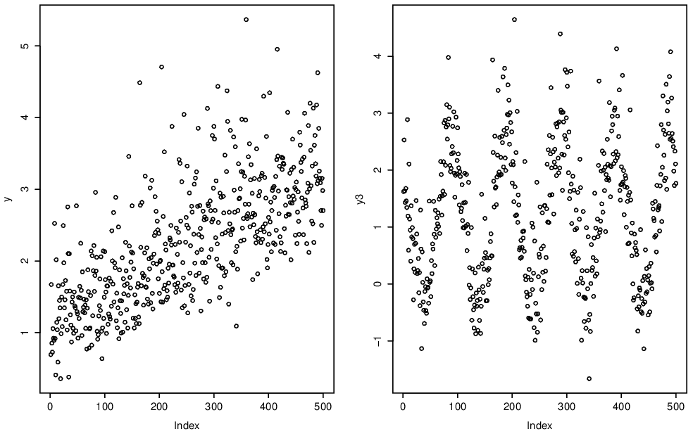
Figure 4.1: Trend in mean.

Trend in variability
Alternatively, we might instead observe some form of trend in the variability of the process. Again the examples we show in Figure 4.2 have linear and cyclic trends in variance.

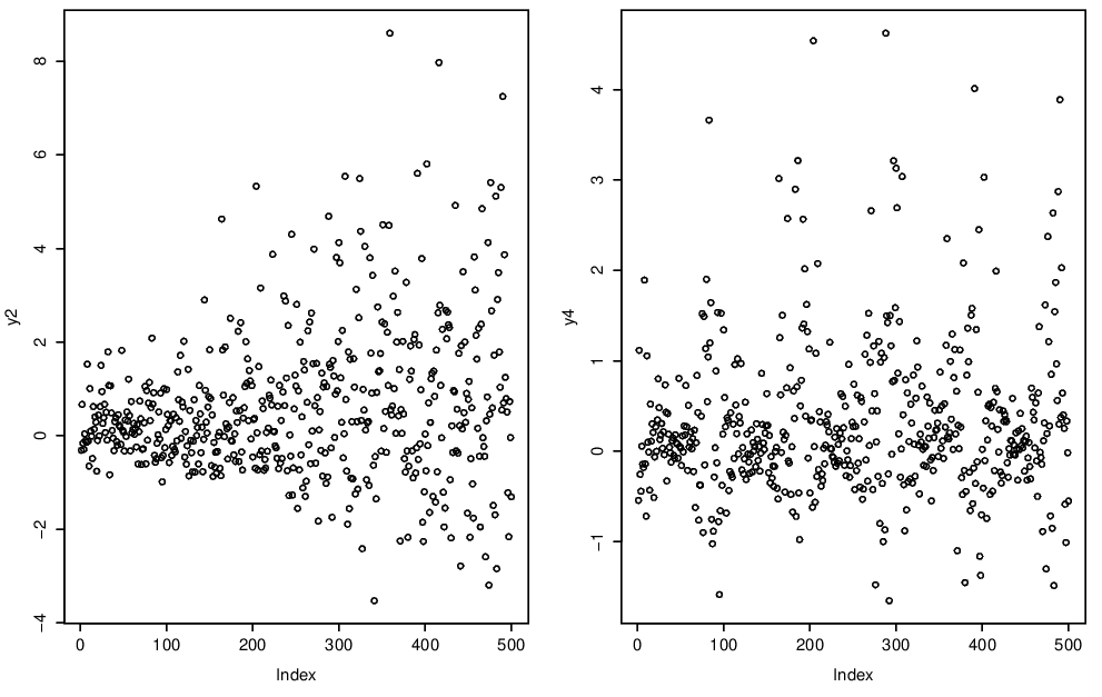
Figure 4.2: Trend in variance.

Notation
Let $\{Y_t\}$ be a non-identically distributed process and let $\{Z_t\}$ be some IID process. We can express trends in the mean and variance of $\{Y_t\}$ as \[\begin{eqnarray} Y_t = Z_t + \alpha(t); \tag{4.1} \end{eqnarray}\] and \[\begin{eqnarray} Y_t = \beta(t) Z_t; \tag{4.2} \end{eqnarray}\] where $\alpha(t)$ and $\beta(t)>0$ are functions of time. Later we see that these can also be functions of covariates which may or may not vary in time. Note that in any practical situation we would observe only the data $\{Y_t\}$ and covariates.

Clearly expressions (4.1) and (4.2) can be combined if the process $\{Y_t\}$ has trends in both mean and variance. In fact, we use these expressions to study the extremes of the observed process $\{Y_t\}$ in Section 4.3.

By defining the non-identically distributed process as a function of a sequence of IID random variables and a deterministic trend it becomes clear how to simulate the processes with trends in mean and/or variance.

First simulate the IID sequence, the examples here use standard Gumbel random variables.
Now add the the trend using equations (4.1) and (4.2) e.g. for a linear trend in mean the required mean function is $\alpha(t)=\alpha_0+\alpha_1 t$.

The simplest method of simulating of the IID sequence is to use the probability integral transform on an IID sequence of standard uniform random variables.

4.1.1 Reading ozone data

Surface-level ozone (O$_3$) levels measured at a site in central Reading are shown in Figure 4.3. Data are daily maxima of hourly observations and are measured in $\mu$gm$^{-3}$. The trends in this data are not so obvious, but there is clearly seasonality - in this case an annual cycle.

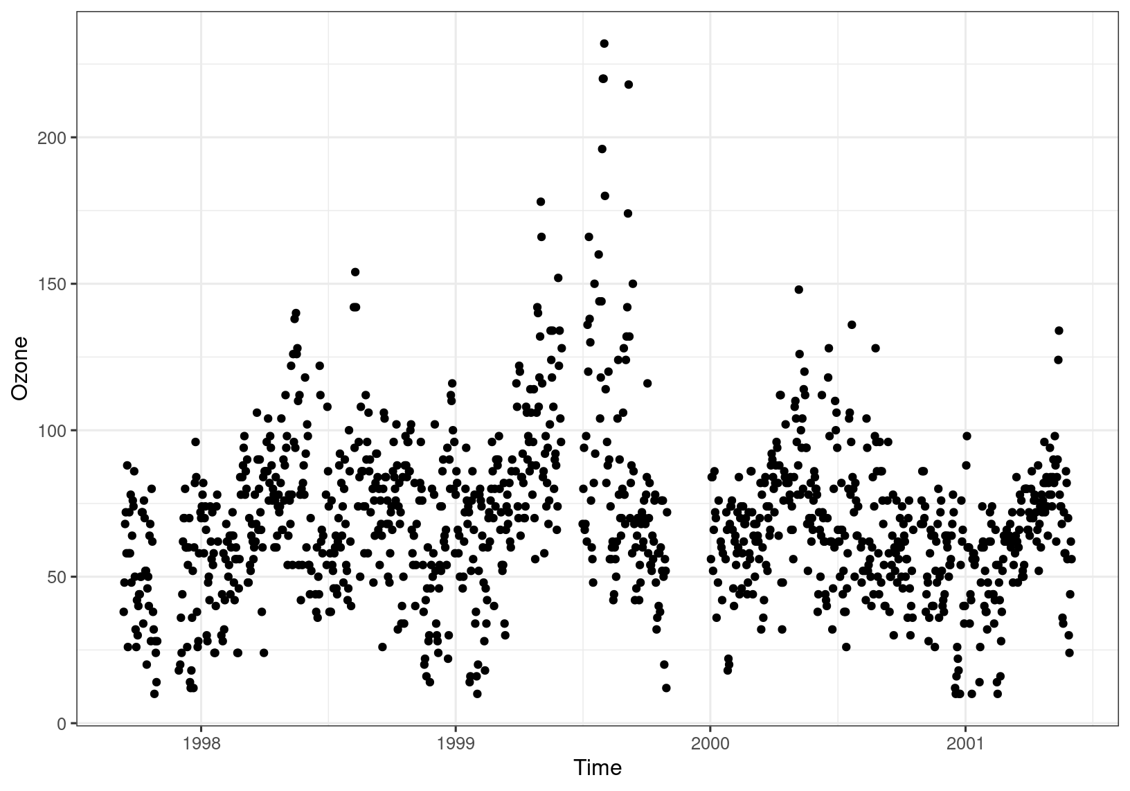
Figure 4.3: Daily maximum ozone in central Reading.

Why is treating a non-identically distributed process as if it were identically distributed unreasonable?

From a statistical point of view, we would be violating the identically distributed part of the IID assumption which will lead to bias in parameter estimates.

From a scientific point of view we would lose vital information about the underlying mechanisms which generate the data which could otherwise be incorporated in a more realistic model.

It is always important to bear in mind what we want to use the model for - forecasting (prediction), an understanding of the mechanisms driving the process or identification of trends. All of these either benefit from or require a model which incorporates non-identical margins.

Scientific notes on Ozone
As discussed above, it is important to have as good an understanding of the scientific background to your data set as possible and to fully understand the uses of a statistical model.

Interesting questions posed in the analysis of ozone include the prediction of high levels of ozone, for public health warnings, and the identification of long-term trends, to assess the impact of legislation to reduce pollution.

Ozone is a secondary pollutant, meaning it is formed in the atmosphere, from precursors (chemicals such as NO$_\mathrm{X}$ and VOC’s) by a series of mostly photochemical (light driven) reactions. Thus meteorological conditions strongly influence the levels of ozone observed. Specifically, ozone levels are high in warm, sunny and still conditions.

4.2 Existing methods for non-identically distributed processes

Existing methods for modelling non-identically distributed processes focus on fitting models with covariates. Specifically, the block maxima, $r$-largest and threshold exceedance models introduced for IID data are maintained, and the non-identical margins are modelled directly through the model parameters.

Covariate models are easily fitted under the likelihood framework and the covariates in the best fitting models are selected using standard methods, e.g. using forward selection and comparing nested models with the likelihood ratio test.

4.2.1 Models for block maxima and $r$-largest

This fitting is straightforward to do and involves iterating through the following steps:

propose linear covariate models for the appropriate parameters of the GEV (the covariate could be time, but could be other explanatory variables depending on the application);
choose a link function for these parameters;
fit the proposed models using maximum-likelihood;
use likelihood methods such as likelihood ratio tests for model selection;
check model fit using standard diagnostic tools such as return level and Q-Q plots.

Examples of possible models are a linear time trend in the mean or a linear time trend in the scale parameter, using the log-link function in the latter: \[\begin{eqnarray*} \mathrm{GEV}(\mu_0+\mu_1t,\sigma,\xi);~~~\mathrm{GEV}(\mu,\exp\{\sigma_0+\sigma_1t\},\xi) \end{eqnarray*}\]

4.2.2 Models for threshold exceedances

The simplest threshold exceedance model for a non-identically distributed process is to split the process into blocks, so that the data within each block is assumed to be IID. The GPD model for IID data is then applied to the data in each block. For example, we could split the Reading ozone data into seasons and analyse each one separately, using the threshold exceedances model.

However, the most common approach takes the threshold exceedances approach and models the non-identical margins directly through the inclusion of covariates in the model parameters, in a similar manner to the covariate models for block maxima and $r$-largest observations. This approach was popularised by the paper of Davison and Smith (1990).

The existing method
The only difference between the existing threshold exceedance approaches for identically and non-identically distributed processes are that families of covariates are incorporated into the GPD and rate parameters in the non-stationary case. We shall denote the covariates associated with $\{Y_t\}$ by $\mathbf{X}_t$. The modelling approach is then

Pick a constant threshold, $u$;
Let $\phi_u=\Pr(Y_t>u)$, then model this exceedance probability by $\phi_u=\phi_u(\mathbf{x}_t)$;
Model the exceedances of $u$ by a GPD distribution with parameters $\sigma_u(\mathbf{x_t})$ and $\xi(\mathbf{x}_t)$.

The rate and GPD scale parameters are forced to lie in the ranges $0 < \phi_u(\mathbf{x}_t) < 1$ and $\sigma_u(\mathbf{x}_t)>0$. In the covariate models we ensure this by using, respectively, logit- and log-link functions. Note also that it is common to assume that the shape parameter $\xi$ is constant, due to the large amount of data needed to model this parameter well. However we continue to think of it as a function of the covariates, in order to work with the most general form of the model.

Functions of the parameters $\phi_u(\mathbf{x}_t),\sigma_u(\mathbf{x_t}),\xi(\mathbf{x}_t)$ are usually taken to be linear functions of the covariates: \[\begin{eqnarray*} \mathrm{logit}~\phi_u(\mathbf{x}_t)=\boldsymbol{\phi}'\mathbf{x}_t,~\log \sigma_u(\mathbf{x}_t)=\boldsymbol{\sigma}_u'\mathbf{x}_t,~\mathrm{and}~\xi(\mathbf{x}_t)=\boldsymbol{\xi}'\mathbf{x}_t. \end{eqnarray*}\] However, other work has looked at fitting non-parametric (Hall and Tajvidi 2000) and additive (Chavez-Demoulin and Davison 2005) models instead. We shall stay within the linear framework.

Inference
We have chosen to work in the likelihood framework under which the non-identically distributed models can be easily fitted. The likelihood for the existing model is \[\begin{eqnarray*} \small L(\boldsymbol{\phi}_u,\boldsymbol{\sigma}_u,\boldsymbol{\xi})=\prod_{t=1}^n (1-\phi_u(\mathbf{x}_t))^{1-I_t} \left(\frac{\phi_u(\mathbf{x}_t)}{\sigma_u(\mathbf{x}_t)}\left[1+\xi(\mathbf{x}_t)\left(\frac{y_t-u}{\sigma_u(\mathbf{x}_t)}\right)\right]_+^{-1/\xi(\mathbf{x}_t)-1}\right) ^{I_t} \end{eqnarray*}\] where $I_t=I[Y_t>u]$ is the indicator function taking the value 1 if the observation is an exceedance and zero otherwise.

The covariates can be selected using standard techniques from linear regression e.g.forward selection in which nested models are compared using the likelihood ratio test.

Return levels
In Section 3.2.6 we looked at estimating return levels for the GEV. The conditional $1/p$ return level for the non-identically distributed GPD model satisfies $\Pr(Y_t > y_{t,p}|\mathbf{X}_t=\mathbf{x}_t) = p$. If $y_{t,p}>u$ and $\phi(\mathbf{x}_t)>p$, this is given by \[\begin{eqnarray*} y_{t,p} = u + \frac{\sigma_u(\mathbf{x}_t)}{\xi(\mathbf{x}_t)}\left[\left(\frac{\phi(\mathbf{x}_t)}{p}\right)^{\xi(\mathbf{x}_t)}-1\right]. \end{eqnarray*}\] To obtain the marginal return level, i.e. $\Pr(Y_t>y_p)=p$, we must integrate out the covariates. In the absence of information on their joint distribution we estimate this empirically so that $y_p$ satisfies \[\begin{eqnarray*} p=\frac{1}{n}\sum_{t=1}^n \phi_u(\mathbf{x}_t)\left[1+\xi(\mathbf{x}_t)\frac{y_p-u}{\sigma_u(\mathbf{x}_t)}\right]_+^{-1/\xi(\mathbf{x}_t)} . \end{eqnarray*}\] This can be solved for $y_p$ using a numerical root-finder.

4.3 Pre-processing method

An alternative method to model the extremes of a non-identically distributed process $\{Y_t\}$ is to pre-process (or pre-whiten) the process to obtain a process that is much closer to the IID assumption than the original one. We then model the extremes of the pre-processed process. This method was developed by Eastoe and Tawn (2009).

The advantages of this method include

computational simplicity;
better interpretability;
greater efficiency;
better theoretical justification.

Pre-processing
Aim: transform the process $\{Y_t\}$ to have identical margins.

One way to do this is to assume the non-identical margins are formed because of a trend in the mean and/or variance, as shown in the examples of section 4.1. We propose going one step further and allow the shape of the underlying marginal distributions of the process to have a trend also. We model this through a Box-Cox parameter $\lambda(\mathbf{x}_t)$.

Recall that $\{Z_t\}$ is an IID process. This model is equivalent to assuming that \[\begin{equation} \frac{Y_t^{\lambda(\mathbf{x}_t)}-1}{\lambda(\mathbf{x}_t)} = \beta(\mathbf{x}_t) Z_t + \alpha(\mathbf{x}_t). \tag{4.3} \end{equation}\]

Having obtained the series $\{Z_t\}$ we model the tails using existing methods;

Pick a constant threshold, $u_z$;
Let $\phi_{z,u}=\Pr(Z_t>u)$, then model this exceedance probability by $\phi_{z,u}=\phi_{z,u}(\mathbf{x}_t)$;
Model the exceedances of $u_z$ by a GPD distribution with parameters $\sigma_{z,u}(\mathbf{x_t})$ and $\xi_z(\mathbf{x}_t)$.

In an ideal world, in which the marginal distribution is perfectly captured in the pre-processing parameters $(\alpha(\mathbf{x}_t),\beta(\mathbf{x}_t),\lambda(\mathbf{x}_t))$ we would not need parameters in the exceedance or GPD covariates. In reality, the pre-processed data will not be IID, perhaps due to missing covariates or because the covariate models are not sensitive enough to pick up subtle relationships, hence the need for covariates.

Inference
Under the likelihood framework this model is simple to fit. First the pre-processing parameters $(\alpha(\mathbf{x}_t),\beta(\mathbf{x}_t),\lambda(\mathbf{x}_t))$ are estimated. There is a range of ways to do this, for simplicity we assume the margins are normal. The process is then transformed using equation (4.3) and the extremes model fitted following the existing method.

Conditional and marginal return levels are found in exactly the same manner as for the existing method, except that they must be back-transformed to the original scale using equation (4.3). Thus if $z_{p,t}$ satisfies $\Pr(Z_t>z_{t,p})=p$ the conditional return levels on the original scale are \[\begin{eqnarray*} y_{t,p}=[\lambda(\mathbf{x}_t)(\beta(\mathbf{x}_t)z_{t,p}+\alpha(\mathbf{x}_t))+1]^{1/\lambda(\mathbf{x}_t)}. \end{eqnarray*}\]

Due to the two-stage nature of the inference procedure of the pre-processing method, confidence intervals for the return levels must be found by bootstrap methods, resampling from the pre-processed data $\{Z_t\}$.

Efficiency
Figure 4.4 compares the efficiency of the existing and pre-processing models for estimating $\alpha_1$ in models $Y_t=Z_t+\alpha(t)$ where

$\alpha(t) = \alpha_0 + \alpha_1 t$ (LHS)
$\alpha(t) = \alpha_0 + \alpha_1 \sqrt 2\cos(\frac{2\pi t}{N}+\frac{\pi}{4})$ (RHS)

In these plots, dashed lines show the expected efficiency loss since the existing method uses only threshold exceedances.

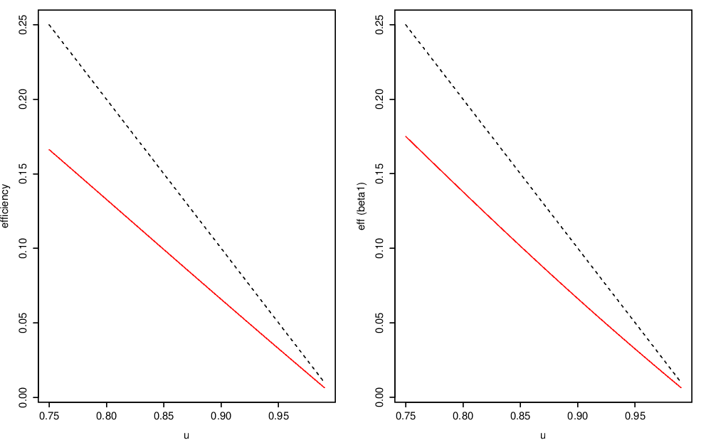
Figure 4.4: Efficiency of pre-processing and existing methods for modelling threshold exceedances

4.4 Analysis of Reading ozone data

We analyse the Reading ozone data using existing and pre-processing methods and compare the results. Following the previous discussion on the science behind the production of atmospheric ozone, we consider daily maxima of NO, NO$_2$ and temperature, aggregate daily sunshine and a year-on-year trend as covariates. We also consider first-order interactions of these. The meteorological data has been obtained from a site situated less than 2km from the air quality monitoring site, courtesy of the UK Met. Office.

We use maximum likelihood estimation throughout and forward selection to choose our covariates.

Figure 4.5 shows the daily maxima of NO ($\mu\mathrm{gm}^{-3}$), NO$_2$ ($\mu\mathrm{gm}^{-3}$) and temperature ($^{\circ}$C) and daily aggregate hours of sunshine.

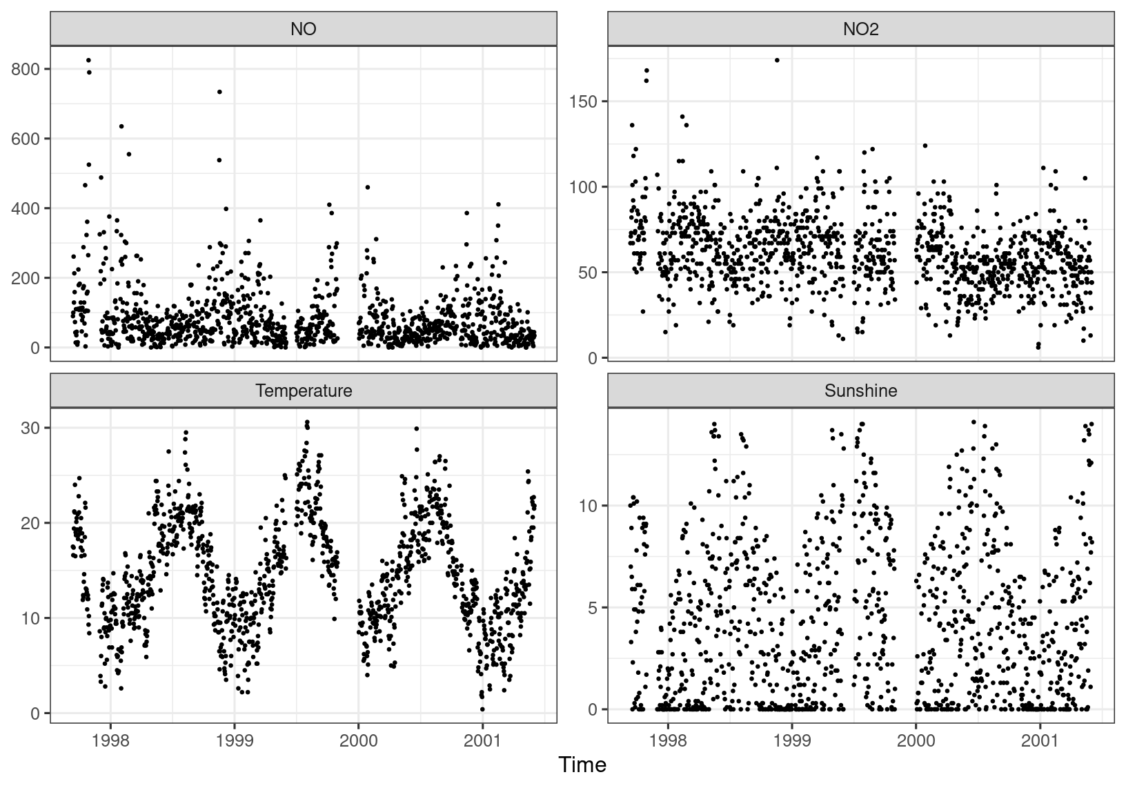
Figure 4.5: Ozone covariates.

Pre-processing parameters
It is standard practise to assume that atmospheric data sets, such as the Reading ozone data, are (log)-normal. In a procedure similar to quasi-likelihood we assume the data to be normal in our estimation of the pre-processing parameters $(\alpha(\mathbf{x}_t),\beta(\mathbf{x}_t),\lambda(\mathbf{x}_t))$. The best fitting models are \[\begin{eqnarray*} \lambda(\mathbf{x}_t) & = & \lambda_0 + \lambda_1 \mathrm{NO}_2 + \lambda_2\mathrm{NO} + \lambda_3\mathrm{Temp} + \lambda_4 \mathrm{Sun} + \lambda_5 \mathrm{Year} \\ &&- \lambda_6\mathrm{NO}_2 \times \mathrm{Temp} - \lambda_7\mathrm{NO}_2 \times \mathrm{Sun} - \lambda_8 \mathrm{Temp}\times \mathrm{Sun}\\ \alpha(\mathbf{x}_t) & = & \alpha_0 + \alpha_1 \mathrm{NO}_2 - \alpha_2\mathrm{NO} + \alpha_3\mathrm{Sun} + \alpha_4\mathrm{NO}_2 \times \mathrm{NO}\\ && -\alpha_5\mathrm{NO}_2 \times \mathrm{Sun} +\alpha_6\mathrm{NO} \times \mathrm{Sun}\\ \log \beta (\mathbf{x}_t) & = & \beta_0 + \beta_1\mathrm{NO} -\beta_2\mathrm{Year}\\. \end{eqnarray*}\]

Thresholds
Figure 4.6 shows the data with the 90% constant (existing method) and varying (pre-processing method) thresholds. Note how closely the varying threshold follows the data.

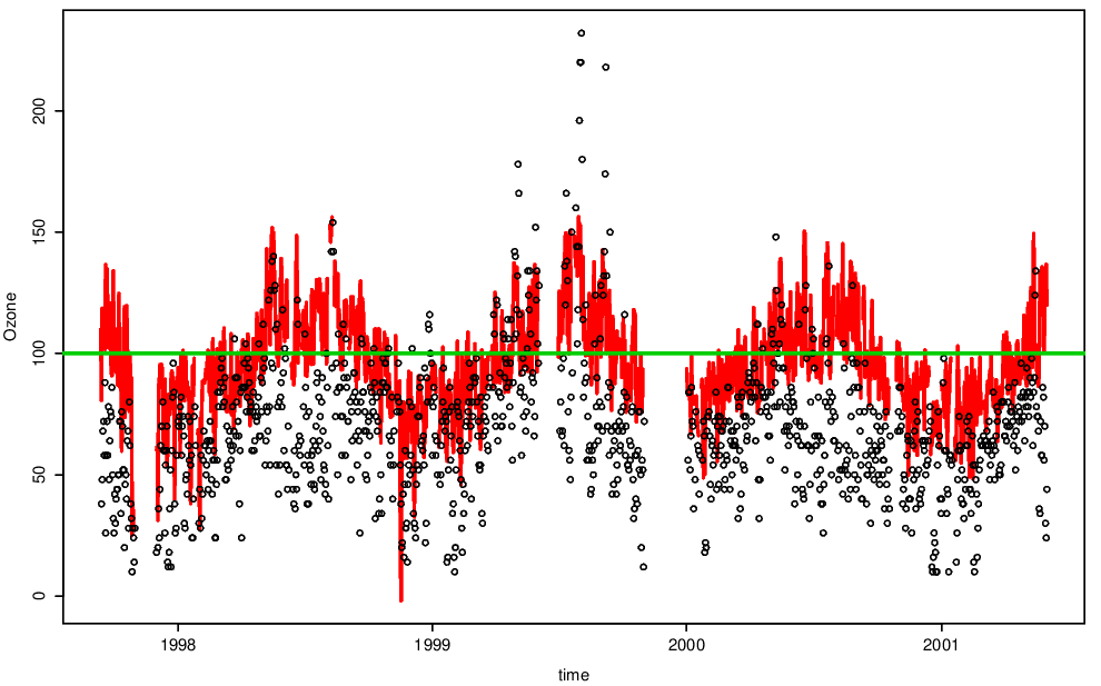
Figure 4.6: Daily maximum ozone with pre-processing threshold shown.

Exceedances parameter
Figure 4.7 shows estimates of the exceedance parameter $\phi_u(\mathbf{x}_t)$. The estimate is constant for the pre-processing method, but extremely variable for the existing method. Notice that the probability of an exceedance under the existing method is also very high ($> 0.5$) in the summer months - are such data really extreme?

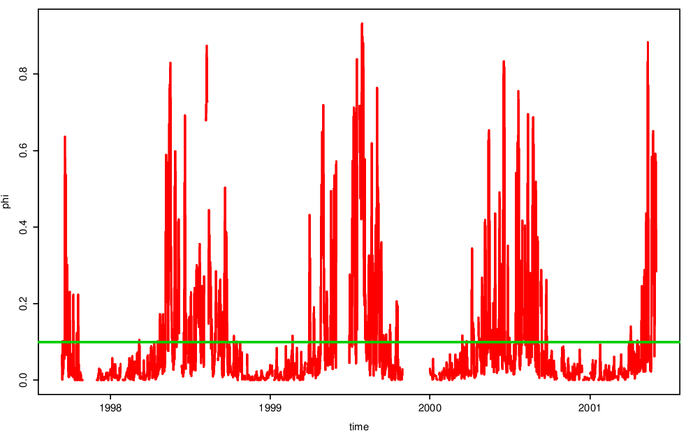
Figure 4.7: Rate parameters for the pre-processing and existing methods for modelling threshold exceedances.

GPD parameters
MLE’s of the parameters in the best fitting model for the exceedances of the 90% threshold using the existing method are \[\begin{eqnarray*} \mathrm{logit}~\phi_{z,u}(\mathbf{x}_t) & = & -5.53-0.0371\mathrm{NO}+0.0127\mathrm{NO}_2+0.137\mathrm{Temp}\\ & & +0.273\mathrm{Sun}+0.000209\mathrm{NO}\times\mathrm{NO}_2;\\ \log \sigma_{z,u} & = & 1.18+0.0848\mathrm{Temp}+0.0578\mathrm{Sun}; \\ \xi(\mathbf{x}_t) & = & -0.337; \end{eqnarray*}\] and using the pre-processing method are \[\begin{eqnarray*} \phi_{z,u}(\mathbf{x}_t) & = & 0.100; \\ \sigma_{z,u} & = & 0.670; \\ \xi(\mathbf{x}_t) & = & -0.192. \end{eqnarray*}\] In this case the pre-processing method results in a much simplified tail model which is therefore much easier to fit.

Conditional return levels
Point estimates (dots) of 99% return levels, with 95% bootstrapped confidence intervals (vertical lines) are shown in Figure 4.8. Crosses denote observed data.

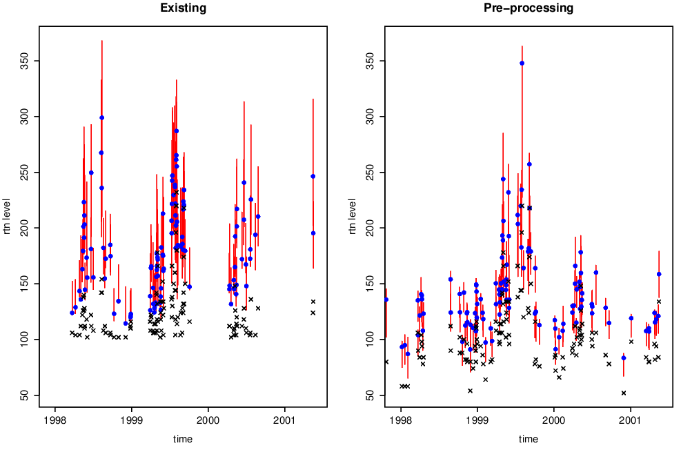
$99\% return levels, with 95\% confidence intervals, from both pre-processing and existing methods. Crosses show observed data.$

Figure 4.8: 99% return levels, with 95% confidence intervals, from both pre-processing and existing methods. Crosses show observed data.

Finally, Figure 4.9 displays box plots of the 95% confidence interval widths for the two methods. The confidence intervals are generally much wider when we use the existing method than when we use the pre-processing method.

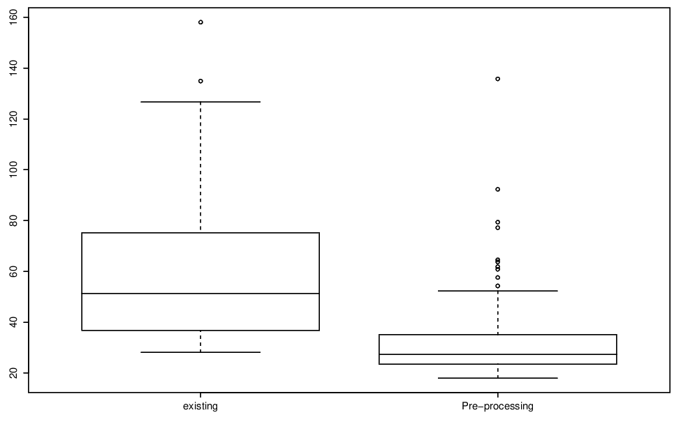
$Boxplots of bootstrapped 95\% confidence intervals of the 99\% return levels shown in previous figure.$

Figure 4.9: Boxplots of bootstrapped 95% confidence intervals of the 99% return levels shown in previous figure.

4.5 Further reading

This paper by Wadsworth, Tawn, and Jonathan (2010) also looked at Box-Cox transform in the context of extremes.

Bibliography

Chavez-Demoulin, V., and A. C. Davison. 2005. “Generalized Additive Modelling of Sample Extremes.” Journal of the Royal Statistical Society: Series C (Applied Statistics) 54 (1): 207–22. https://doi.org/10.1111/j.1467-9876.2005.00479.x.

Davison, A. C., and R. L. Smith. 1990. “Models for Exceedances over High Thresholds.” Journal of the Royal Statistical Society B 52 (3): 393–442.

Eastoe, Emma F., and Jonathan A. Tawn. 2009. “Modelling Non-Stationary Extremes with Application to Surface Level Ozone.” Journal of the Royal Statistical Society. Series C (Applied Statistics) 58 (1): 25–45. http://www.jstor.org/stable/25578145.

Hall, P., and N. Tajvidi. 2000. “Nonparametric Analysis of Temporal Trend When Fitting Parametric Models to Extreme-Value Data.” Statistical Science 15 (2): 153–67.

Wadsworth, J. L., J. A. Tawn, and P. Jonathan. 2010. “Accounting for Choice of Measurement Scale in Extreme Value Modeling.” The Annals of Applied Statistics 4 (3): 1558–78. http://www.jstor.org/stable/29765567.

Lancaster University MATH456/556