7 Extremes in Finance
In this chapter, we look at methods in extreme value theory that are suitable for applications to financial data. However, it should not be mistaken that they are not applicable to other kinds of data e.g. environment data.
7.1 The Hill estimator for heavy-tailed data
Financial data almost always have heavy tails \((\xi>0)\). Sometimes a simpler model is assumed for the survivor function, which is a good approximation to the GPD for large values. We assume \[\begin{eqnarray} \Pr(X>x) \approx \frac{c}{x^{\alpha}},~~~c>0, \alpha>0, x>u, \tag{7.1} \end{eqnarray}\] for \(u\) a high threshold. Thus we have \[\begin{eqnarray} \Pr(X>x|X>u) \approx (u/x)^\alpha. \tag{7.2} \end{eqnarray}\] This model is very similar to the GPD for \(\xi>0\) and large \(x\).
We begin with the GPD expression for \(\Pr(X>x|X>u)\): \[\begin{align*} \left[1+\xi \left(\frac{x-u}{\sigma_u}\right)\right]_+^{-1/\xi} & = \left(\frac{\sigma_u}{\xi}\right)^{1/\xi} x^{-1/\xi} \left[1+\frac{\sigma_u-\xi u}{\xi x}\right]^{-1/\xi}\\ & = \left(\frac{\sigma_u}{\xi}\right)^{1/\xi} x^{-1/\xi}[1+O(x^{-1})],~~x\to\infty \end{align*}\] Now \(\sigma_u = \sigma+\xi(u-\mu)\), so \(\sigma_u-\xi u\) does not depend on \(u\) and furthermore \[\begin{eqnarray*} \left(\frac{\sigma_u}{\xi}\right)^{1/\xi} = u^{1/\xi}\left(1+\frac{\sigma/\xi-\mu}{u}\right)^{1/\xi} \approx u^{1/\xi} \end{eqnarray*}\] for large \(u\). Therefore \(\Pr(X>x|X>u) \approx (u/x)^{1/\xi}\), for large \(x\) and large \(u\), which is the expression (7.2) for \(\alpha=1/\xi\).
7.1.1 The Hill estimator of \(\alpha\)
The advantage of equation (7.1) is it lends itself to a simple, closed form estimator for \(\alpha\) (equivalently \(\xi\)). Although numerical methods now make maximisation of GPD likelihoods very simple, the Hill estimator is still widely used by many who work with heavy-tailed data. There is more than one way to derive the estimator: we shall stick with a likelihood motivation.
According to (7.1), the density for an observation, given that it exceeds \(u\), is \[\begin{eqnarray*} f(x|X>u) = \alpha u^{\alpha} x^{-\alpha-1}. \end{eqnarray*}\] For a total of \(n_u\) threshold exceedances, this gives the MLE of \(\alpha\) as \[\begin{eqnarray*} \hat{\alpha} = \left[\frac{1}{n_u} \sum_{i=1}^{n_u} (\log x_i - \log u)\right]^{-1}. \end{eqnarray*}\] Often the threshold \(u\) is actually taken to be the \(k\)-th order statistic, \(X_{(k)}\). The choice of \(k\) is similar to the choice of \(u\), in the sense of the bias-variance trade-off involved.
7.1.2 Estimation of \(c\)
Estimation of \(c\) can be performed by using the empirical proportion of exceedances to estimate the theoretical proportion: \[\begin{eqnarray*} \Pr(X>u) = \frac{c}{u^{\alpha}} =\frac{n_u}{n} \end{eqnarray*}\] so \(\hat{c} = \frac{n_u}{n} u^{\hat{\alpha}}\). Plugging in the estimated \(\hat{\alpha}\), \(\hat{c}\) into equation (7.1) provides a simple estimate of high quantiles. \[\begin{eqnarray*} x_p = \left(\frac{p}{\hat{c}}\right)^{-1/\hat{\alpha}}. \end{eqnarray*}\]
7.2 Modelling dependence
Suppose we are interested in the risk associated to more than one stock. Tho assess this we need to model the dependence between the stocks at extreme levels.
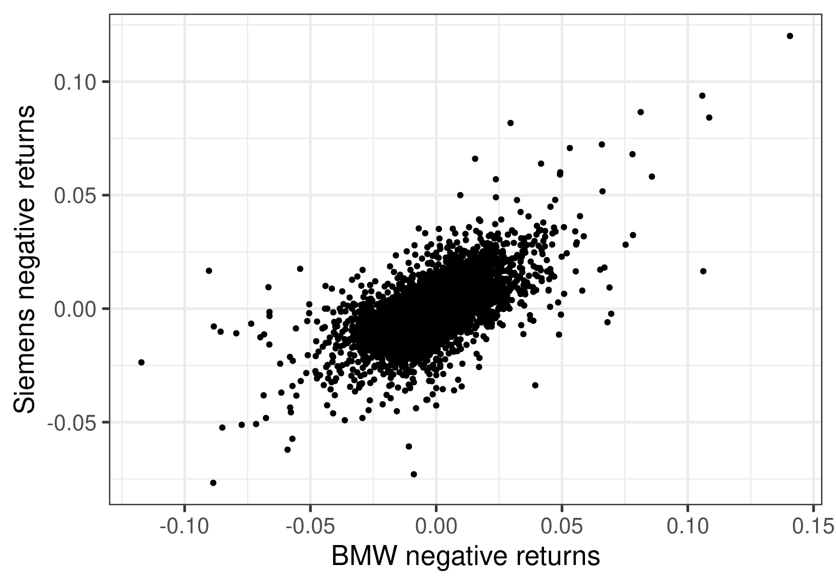 The figure shows the negative returns of BMW plotted against the negative returns of Siemens over the same period. There is a positive relationship, and we need to take this into account in calculating the risk of a portfolio containing both of these stocks.
7.2.1 Correlation
The first measure of dependence people usually think of is correlation. \[ \begin{aligned} \mbox{Corr}(X,Y) = \frac{E(XY)-E(X)E(Y)}{\sqrt{\mbox{Var}(X)}\sqrt{\mbox{Var}(Y)}} \end{aligned} \] This measure:
- Requires existence of first and second moments
- Is not invariant to marginal choice
- Only fully characterises the dependence if \((X,Y)\) have a bivariate Gaussian distribution.
7.2.2 Alternative dependence measures
Fitting a bivariate Gaussian distribution to the data with the estimated correlation coefficient is as arbitrary as fitting a Gaussian model to the margins and using the estimated tail for the extremes.
As in the univariate case, we anticipate that dependence at extreme levels is different to that at “average” levels. We don’t want to contaminate our estimate of extremal dependence with average dependence.
7.2.2.1 Motivating examples
Let us assume that our variables have standard Fréchet margins, so \(\Pr(X\leq x) = e^{-1/x}\). As \(x\to\infty\), \[\begin{eqnarray*} \Pr(X>x) = x^{-1}[1+O(x^{-1})]. \end{eqnarray*}\]
Independence
If \((X,Y)\) are independent then their joint survivor function evaluated on the diagonal can be expressed as
\[\begin{eqnarray*}
\Pr(X>x,Y>x) = x^{-2}[1+O(x^{-1})]~~x\to\infty.
\end{eqnarray*}\]
Bivariate extreme value distribution
If \(\Pr(X\leq x, Y\leq y) = \exp\{-V(x,y)\}\) with \(V:(0,\infty)^2\to(0,\infty)\) homogeneous of order 1 we say \((X,Y)\) have a bivariate extreme value distribution. Then
\[\begin{eqnarray*}
\Pr(X>x,Y>x) = x^{-1}[2-V(1,1)+O(x^{-1})],~~x\to\infty.
\end{eqnarray*}\]
Bivariate normal distribution
If \((\Phi^{-1}(\exp\{-1/X\}), \Phi^{-1}(\exp\{-1/Y\})) \sim\) N\(_2(\rho)\) then
\[\begin{eqnarray*}
\Pr(X>x,Y>x) = x^{-2/(1+\rho)}[C_{\rho} (\log(x))^{\rho/(1+\rho)}+o(1)],~~x\to\infty.
\end{eqnarray*}\]
7.2.3 The coefficient of tail dependence
Let us assume that our variables have standard Fréchet margins (achieved by a transformation). Then a very general assumption is \[\begin{eqnarray} \Pr(X>x, Y>x) = L(x)x^{-1/\eta},~~~x\to \infty, \tag{7.3} \end{eqnarray}\] where
- \(L:(0,\infty)\to (0,\infty)\) is termed a slowly varying function3
- \(\eta \in(0,1]\) is the coefficient of tail dependence
Values of \(\eta\) close to 0 indicate weak (negative) extremal dependence, \(\eta=1/2\) corresponds to near independence, and \(\eta\) near 1 corresponds to strong extremal dependence.
Let us suppose that \(L(x) \approx C\), since slowly varying functions do not change much over a large range of \(x\). We can rewrite equation (7.3) as \[\begin{eqnarray*} {\Pr(\min(X,Y)>x) \approx Cx^{-1/\eta}}. \end{eqnarray*}\] Note the similarity with equation (7.1). We can use the Hill estimator to estimate \(\eta\).
For an interpretation of \(\eta\), consider the conditional probability \[\begin{eqnarray*} \Pr(X>x | Y>x) \approx Cx^{1-1/\eta}. \end{eqnarray*}\] If \(\eta=1\) this probability is constant irrespective of the value of \(x\) (as long as \(x\) is large). Otherwise it decreases with \(x\), and this decrease is more rapid more smaller \(\eta\).
7.2.4 Example: dependence in negative returns
The first stage in the estimation is to transform the margins to standard Fréchet. We need the Probability Integral Transform (Section 3.2.5).
If \(X \sim F\), then \(-1/\log F(X) \sim\) Fréchet. Thus we need an estimate of \(F\). We could either
- Use the empirical distribution function (EDF) throughout
- Use the EDF up to a threshold \(u\), and the GPD above the threshold
Option 1 means setting: \[\begin{eqnarray*} \tilde{F}(X_i) = \mbox{rank}(X_i)/(n+1). \end{eqnarray*}\] For Option 2, above a threshold \(u\), we set \[\begin{eqnarray*} \hat{F}(X_i) = 1-\hat{\phi}_u[1+\hat{\xi}(X_i-u)/\hat{\sigma}_u]^{-1/\hat{\xi}}_+. \end{eqnarray*}\]
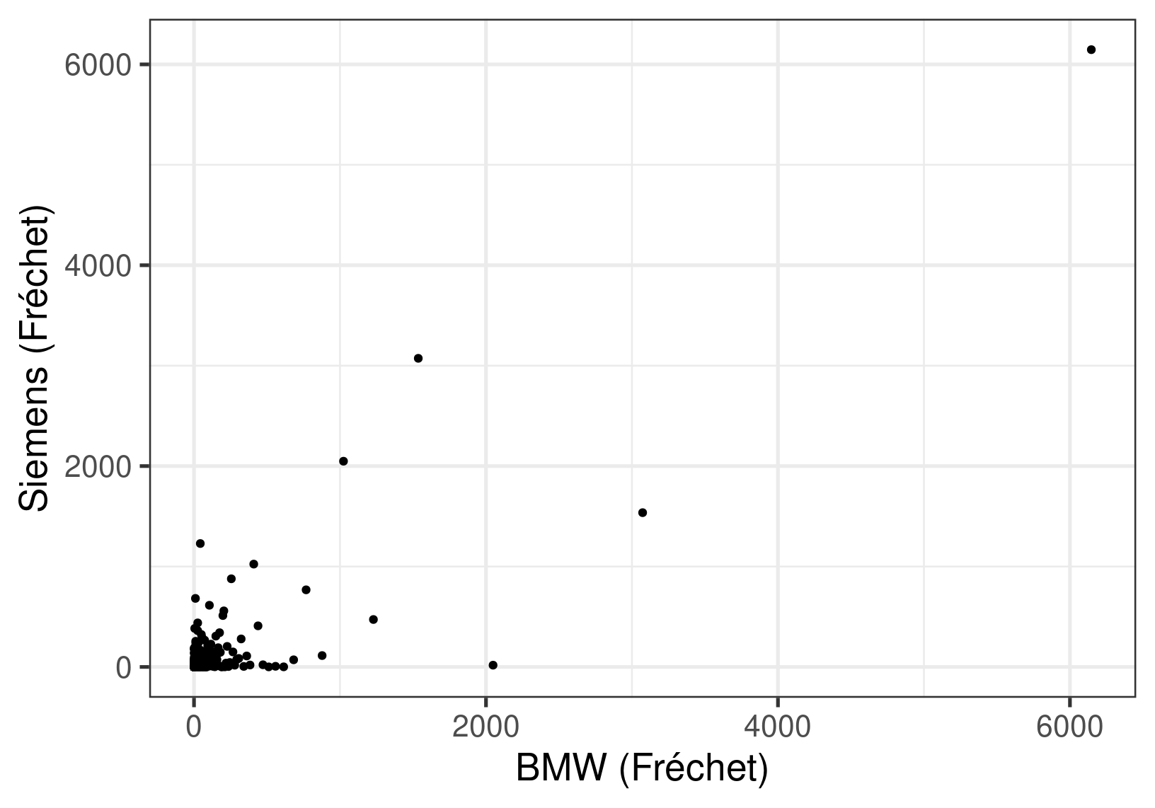 Set \(Z_i = \min(X_i,Y_i)\)
\[\begin{eqnarray*}
\hat{\eta} = \frac{1}{n_u} \sum_{i=1}^{n_u} (\log z_i - \log u)
\end{eqnarray*}\]
For \(u\) equal to the 0.95 quantile of the \(Z_i\) we have \(\hat{\eta} = 0.916\) (standard error 0.055), suggesting fairly strong extremal dependence.
We can now estimate the level of the loss that is exceeded by both variables with small probability \(p\). \[\begin{eqnarray*} \Pr(\min(X,Y)>z_p) \approx \hat{C} z_p^{-1/\hat{\eta}} = p, \end{eqnarray*}\] using the estimate of \(C\) as in Section 7.1.2. To translate the estimated \(z_p\) back to the returns scale we need to use the inverse of the earlier transformation to the Fréchet scale. This, amongst other reasons, suggests use of Option 2 is preferable for the transformation.
7.2.5 The extremal index and the coefficient of tail dependence
The coefficient of tail dependence \(\eta\) describes the dependence in the extreme values of two random variables. This is different to what we have seen in Chapter 5.3, where the extremal index \(\theta\) describes the short-range temporal/serial dependence in the extreme values of stationary processes. Their difference is analogous to that between the Pearson correlation of two variables (Chapter 7.2.1) & the autocorrelation function of a time-series.
It is possible to investigate both kinds of dependence for the same set of variables. For example, we consider the variables \(\{X_t\}\) in a stationary (but dependent) process, where we can calculate the extremal index as usual. We can also compute the coefficient of tail dependence by considering \(\{X_t\}\) and \(\{X_{t-1}\}\) as the two variables of interest.
7.2.6 Multivariate extremes and further reading
The coefficient of tail dependence can be extended to a multivariate setting and computed for all possible pairs of random variables. As multivariate extremes are beyond this module’s scope, we will include some references here. The original proponents of \(\eta\) are Ledford and Tawn (1996) and Ledford and Tawn (1998), while Heffernan (2000) provided a comprehensive directory of \(\eta\) for different bivariate distributions. Other related works include, in chronological order, Sibuya (1960), Mardia (1964), Tiago de Oliveira (n.d.), Pickands (1981), Coles and Tawn (1991), Ledford and Tawn (1997), and Coles, Heffernan, and Tawn (1999). A general reference on multivariate models and dependence concepts is Joe (1997). Finally, Heffernan and Tawn (2004) proposed a different yet influential conditional approach to multivariate extremes.
7.3 Value at Risk, Expected Shortfall, & Volatility
You may also have learned about Value at Risk (VaR), which is indeed equivalent to high quantiles and return levels we have seen in Section 2.3.3. In this section, we will look deeper into VaR & a related quantity called Expected Shortfall (also known as Conditional VaR), and the effect of volatility in the calculations of VaR.
7.3.1 Fitting GEV
Often in financial contexts, one is more concerned with the loss in a particular day, rather than the maximum losses over a particular time period (e.g. three months). How can we use the models we have learned to help with this estimation?
Recall that, for an IID sequence \(\{X_t\}\) assumed to come from the distribution \(F\), \[ \Pr(M_n\leq y)=F(y)^n\approx G\left(\frac{y-b_n}{a_n}\right), \] where \(M_n\) is the block maxima of size \(n\) (e.g. maxima of \(n\) daily negative returns), and our estimated GEV distribution, \(G\left(\frac{y-b_n}{a_n}\right)=\tilde{G}(y)\) is approximately \(F(y)^n\). One way to translate our return levels to quantiles of the original distribution is to solve \[ F(z_p)=\tilde{G}^{1/n}(z_p)=p \] giving \[ z_p=\mu-\frac{\sigma}{\xi}\left[1-\left(-n\log p\right)^{-\xi}\right]. \] Compare this to Equation (2.6). When referring to daily negative returns, this quantity is called the \(100p\)% VaR, which is the value that will be exceeded with probability \(1-p\). That is, for a series of negative daily returns, \(X_t\), \[ \Pr(X_t\leq\mbox{VaR}(p))=p \qquad \Leftrightarrow \qquad \Pr(X_t>\mbox{VaR}(p))=1-p. \] Note that, the definition of VaR\((p)\) varies slightly in the literature, as, for example, the 99% VaR here may be called the 1% VaR elsewhere. Nevertheless, there usually is no ambiguity as investors are most interested in large potential losses.
BMW exampleWe continue with the daily negative returns seen above, but focus on one of the two stocks, namely BMW.
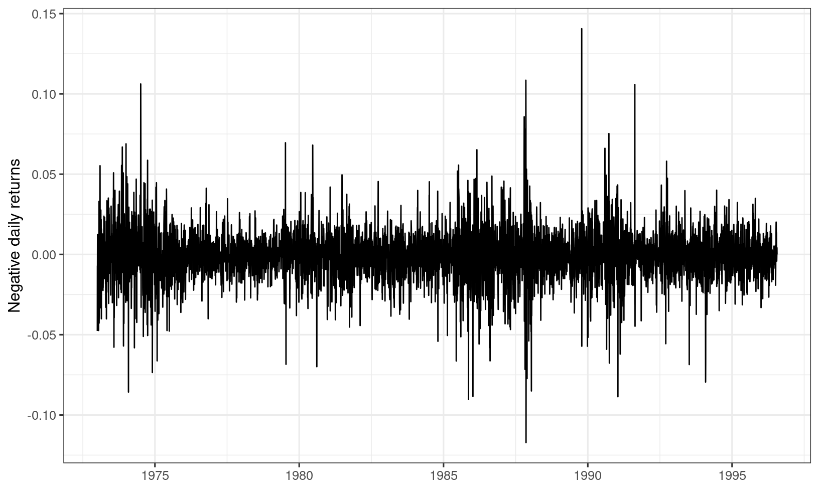
Figure 7.1: Daily negative returns of BMW.
The BMW data were maxima of \(n=66\) consecutive negative returns (which is approximately three months of trading days). There were \(g=93\) such maxima, so the maxima relate to a total of \(T=ng=6138\) daily negative returns.
The \(95\)% VaR (that is, the negative return value that will be exceeded with probability \(5\)% on a given day) is \[\begin{eqnarray*} \hat\mu -\frac{\hat\sigma}{\hat\xi}\left[1-\{-66\log(0.95)\}^{-\hat\xi}\right] = 0.0153 \end{eqnarray*}\]
The \(99\)% VaR is \[\begin{eqnarray*} \hat\mu -\frac{\hat\sigma}{\hat\xi}\left[1-\{-66\log(0.99)\}^{-\hat\xi}\right] = 0.0333 \end{eqnarray*}\]
To obtain estimates of uncertainty, we could again use the delta method or profile likelihood.
7.3.2 Fitting GPD & undoing the conditioning
Suppose we fit the GPD to a series of negative returns. How do we calculate the VaR? We know \[\begin{eqnarray*} \Pr(X> x | X>u) = \left[1+\xi\left(\frac{x-u}{\sigma_u}\right)\right]^{-1/\xi}_+. \end{eqnarray*}\] We need to undo the conditioning to calculate the quantile.
The GPD provides a model for excesses conditional upon being an excess. We undo this conditioning by modelling the number of exceedances, \(N_u\), assuming either
- \(N_u \sim\) Poisson\((\gamma_u), ~~~ \gamma_u = E(N_u)\)
- \(N_u \sim\) Binomial\((n,\phi_u), ~~~ \phi_u=\Pr(X>u)\)
The first option is equivalent to the Poisson process model of Section 3.1.4, with a different parameterisation. The second is almost equivalent for large sample sizes. The maximum likelihood estimate for \({\phi_u}\) is \({n_u/n}\), with \({N_u=n_u}\) the observed number of exceedances of \(u\), from a total of \(n\) data points. VaR\((p)\) can thus be found by solving \[\begin{eqnarray*} 1-\left[1+\hat\xi\left(\frac{\mbox{VaR}(p)-u}{\hat\sigma_u}\right)\right]^{-1/\hat\xi} \hat\phi_u = p \end{eqnarray*}\] to give \[\begin{eqnarray*} \mbox{VaR}(p) = u +\frac{\hat\sigma_u}{\hat\xi}\left[\left(\frac{\hat\phi_u}{1-p}\right)^{\hat\xi}-1\right]. \end{eqnarray*}\]
BMW example
We continue with the BMW example. We choose \(u = 0.03\), which means there are \(136\) exceedances (quite comparable to the number of block maxima). Using the parameter estimates, we can calculate the \(95\)% VaR:
\[\begin{eqnarray*}
u + \frac{\hat\sigma_u}{\hat\xi}\left[\left(\frac{\hat\phi_u}{1-0.95}\right)^{\hat\xi}-1\right] = 0.0203
\end{eqnarray*}\]
The \(99\)% VaR is
\[\begin{eqnarray*}
u + \frac{\hat\sigma_u}{\hat\xi}\left[\left(\frac{\hat\phi_u}{1-0.99}\right)^{\hat\xi}-1\right] = 0.0406
\end{eqnarray*}\]
We can see the estimated VaRs are similar but slightly larger than those by using the GEV for block maxima.
7.3.3 Expected Shortfall
Expected Shortfall, \({\mbox{ES}(p)}\), also known as conditional VaR, is the name given to the expected negative return, given that the VaR threshold has been exceeded. If \({X}\) denotes a negative return then \[\begin{eqnarray*} \mbox{ES}(p) = E[X|X>\mbox{VaR}(p)]. \end{eqnarray*}\] Assuming \(\mbox{VaR}(p)\) to be a high threshold, and we have fitted a GPD above a threshold \({u<\mbox{VaR}(p)}\), this is calculated using the expression in Section 3.2.2. \[\begin{align*} \mbox{ES}(p) &= \mbox{VaR}(p) + \frac{\sigma_v}{1-\xi},\qquad\qquad\qquad(\mbox{where}~v=\mbox{VaR}(p))\\ &= \mbox{VaR}(p) + \frac{\sigma_u + \xi(\mbox{VaR}(p) - u)}{1-\xi}. \end{align*}\]
7.3.4 Adjustment to VaR for dependent data
Thus far we have ignored dependence in our VaR calculations. We have seen two methods for calculating VaR:
- Fitting the GEV to “subperiod maxima” (e.g. three-monthly maxima) and solving \(\tilde{G}^{1/n}(z_p) \approx F(z_p) = p\)
- Fitting the GPD to all exceedances and solving \(P(X>z_p|X>u)\phi_u \approx 1-F(z_p) = 1-p\)
with \(z_p = \mbox{VaR}(p)\).
How do we calculate the VaR when it is evident that there is serial dependence in the data?
Adjusting for subperiod maxima
As seen in Section 5.3.2 our estimated GEV for a stationary process is \(\tilde{H}(x)\approx F(x)^{n\theta}\). Thus we need to solve \({\tilde{H}^{1/(n\theta)}(z_p) = p}\):
\[\begin{eqnarray*}
\hat{z_p}=\hat\mu -\frac{\hat\sigma}{\hat\xi}\left[1-\{-n\theta\log p\}^{-\hat\xi}\right]
\end{eqnarray*}\]
with \(z_p = \mbox{VaR}(p)\). If \(\theta<1\) this estimate is larger than when \(\theta=1\). Ignoring dependence thus means we underestimate the VaR. Note that we will still need all data to estimate the extremal index (via the Runs Method).
Adjusting for all exceedances
The original estimate is still valid in this case. However, if we use all exceedances to estimate parameters, then an adjustment to the standard errors would be required (cf. Section 6.2).
BMW example
Going back to previous results, the estimates of the GPD parameters for the entire series taking a threshold of \(u=0.03\) are \(\hat{\sigma}_u=0.0126~(0.00157)\) and \(\hat{\xi} = 0.143~(0.0947)\). The quoted standard errors are too small as the exceedances are not independent.
The estimates of the GPD parameters using clustering maxima for clusters defind by the runs method taking \(u=0.03\) and \(m = 10\) are \(\hat{\sigma}_u=0.0126~(0.00189)\) and \(\hat{\xi} = 0.179~(0.116)\). These standard errors are more reliable.
The \(99\)% VaR for the three monthly maxima of these data was estimated as \(0.0333\). However, this estimate didn’t take account of the dependence, measured via the extremal index \(\theta\), estimated in Figure 7.2.
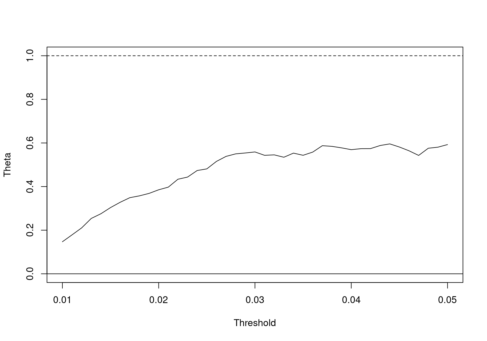
Figure 7.2: Runs estimate of the extremal index for BMW data.
A threshold of \(u=0.03\) and run length \(m = 10\) appears to give a stable estimate of \(\hat{\theta} \approx 0.593\). Including this in the VaR\((0.99)\) calculation gives \[ \hat\mu -\frac{\hat\sigma}{\hat\xi}\left[1-\{-0.593 \times 66 \log(0.99)\}^{-\hat\xi}\right] = 0.0406 \] which is exceeded by a proportion of \(0.0103\) of the data, and closer to the estimate according to the GPD approach.
7.3.5 Volatility
In Section 6.1.1.1, we saw that whether or not we account for volatility makes a difference to our analysis. Thus far we have calculated VaR as a quantile of the entire series over a long time period, ignoring the local variation, which is however usually present in financial time series (see, for example, Figure 7.1). In practice, we may want to estimate VaR for tomorrow rather than on an arbitrary day.
One approach to removing volatility is similar to that seen in Section 6.1.1.1 . Define the filtered negative returns by \[\begin{eqnarray*} Z_t = \frac{X_t - \tilde{E}(X_t)}{\tilde{SD}(X_t)} \end{eqnarray*}\] where \(\tilde{E}(X_t)\) and \(\tilde{SD}(X_t)\) are local estimates of the mean and standard deviation, for example using the sample mean and sample standard deviation of the previous \(h\) observations.
Suppose that we have a series of length \(T\). The VaR for the day \(T+1\) can be estimated as \[\begin{eqnarray*} \mbox{VaR}(p)[T+1] = \mbox{VaR}_{Z}(p)\times \tilde{SD}(X_T) + \tilde{E}(X_T) \end{eqnarray*}\] where \({\mbox{VaR}_{Z}(p)}\) is the VaR estimated from the filtered series \(Z_t\).
BMW example
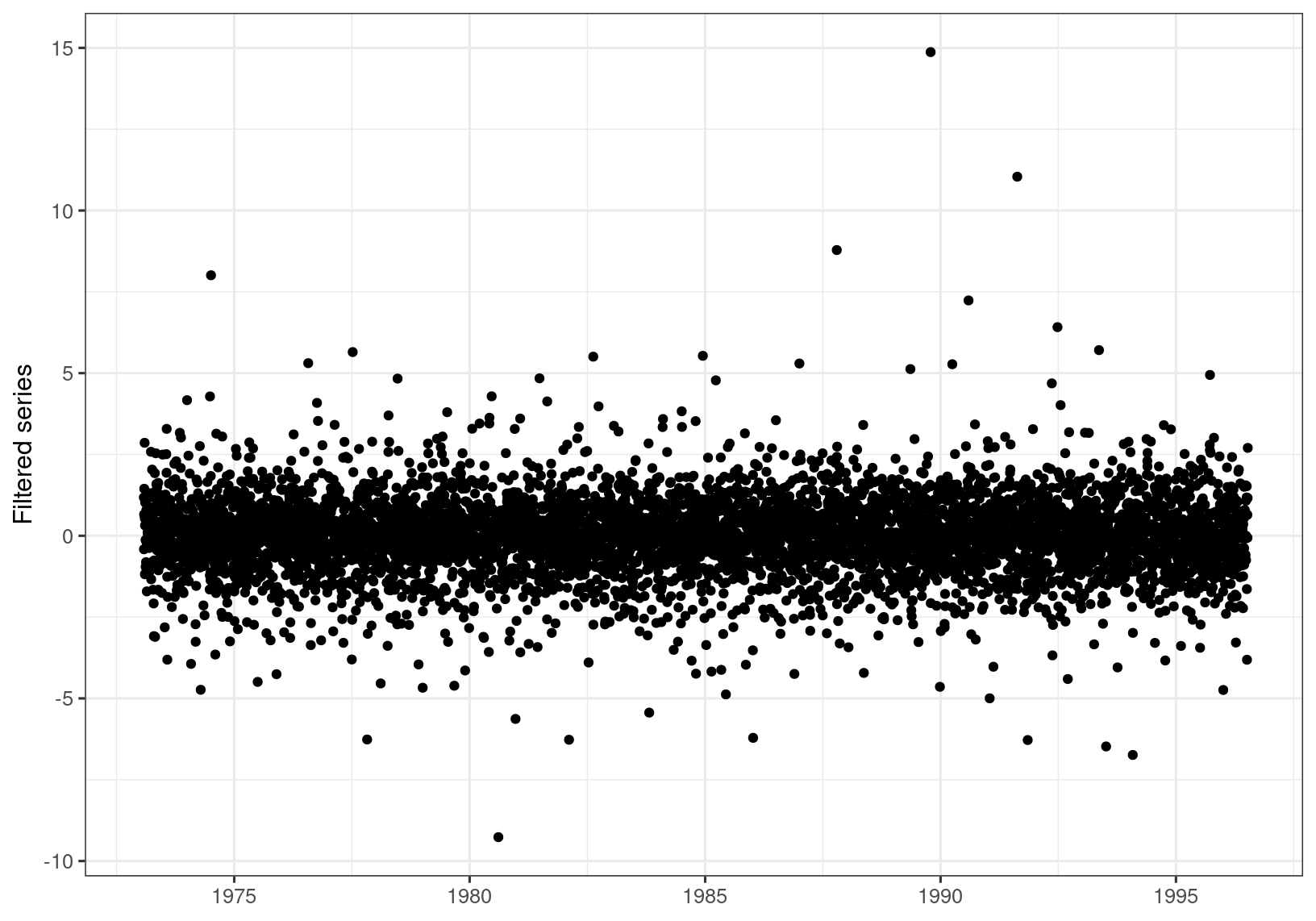
Figure 7.3: Filtered series for BMW data.
We will calculate VaR\((p)[t]\) for \(t\geq h\), with \(h = 20\). First we obtain the filtered series, which is shown in Figure 7.3.
Following the usual procedure the \(\text{VaR}(0.99)\) is estimated as \(3.06\). Transforming to the return series gives the following plot of daily \(99\)% VaR estimates
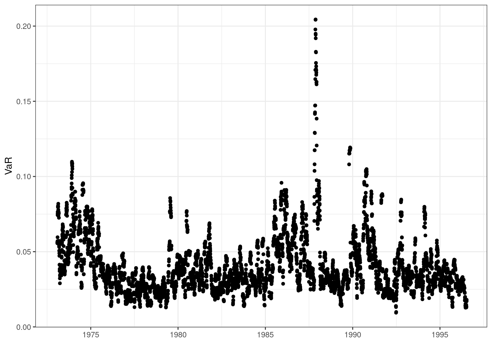 The proportion of data exceeding \(\text{VaR}(0.99)[t]\) is (interestingly) \(0.0105\), while the proportion of data exceeding \(\text{VaR}(0.99)\) is \(0.0103\). Both are correct in the long run.
7.4 Volatility models
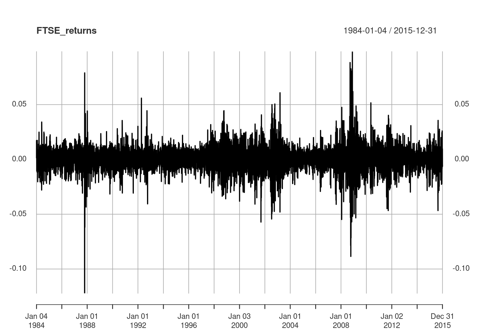
Figure 7.4: Returns of the FTSE index.
You may have learned about (G)ARCH and other models that account for the volatility directly. Here, we will be using the GARCH\((1,1)\) model as an example for the FTSE return series in Figure 7.4, denoted by \(\{X_t\}\). The model equations are \[\begin{align*} X_t &= \sigma_t\epsilon_t, \\ \sigma_t^2 &= \omega + \alpha X_{t-1}^2 + \beta \sigma_{t-1}^2, \end{align*}\] where \(\omega>0,\alpha\geq0,\beta\geq0\), and the innovation series \(\{\epsilon_t\}\) are IID with expectation 0 and variance 1. It is also usually assumed that the innovations are normally distributed.
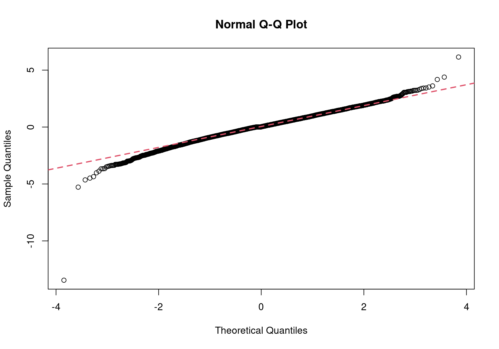
We examine if the normality assumption is reasonable after fitting to the FTSE data. From the Q-Q plot of the residuals, which are proxies of the innovation sequence, we can safely say they are not normally distributed.
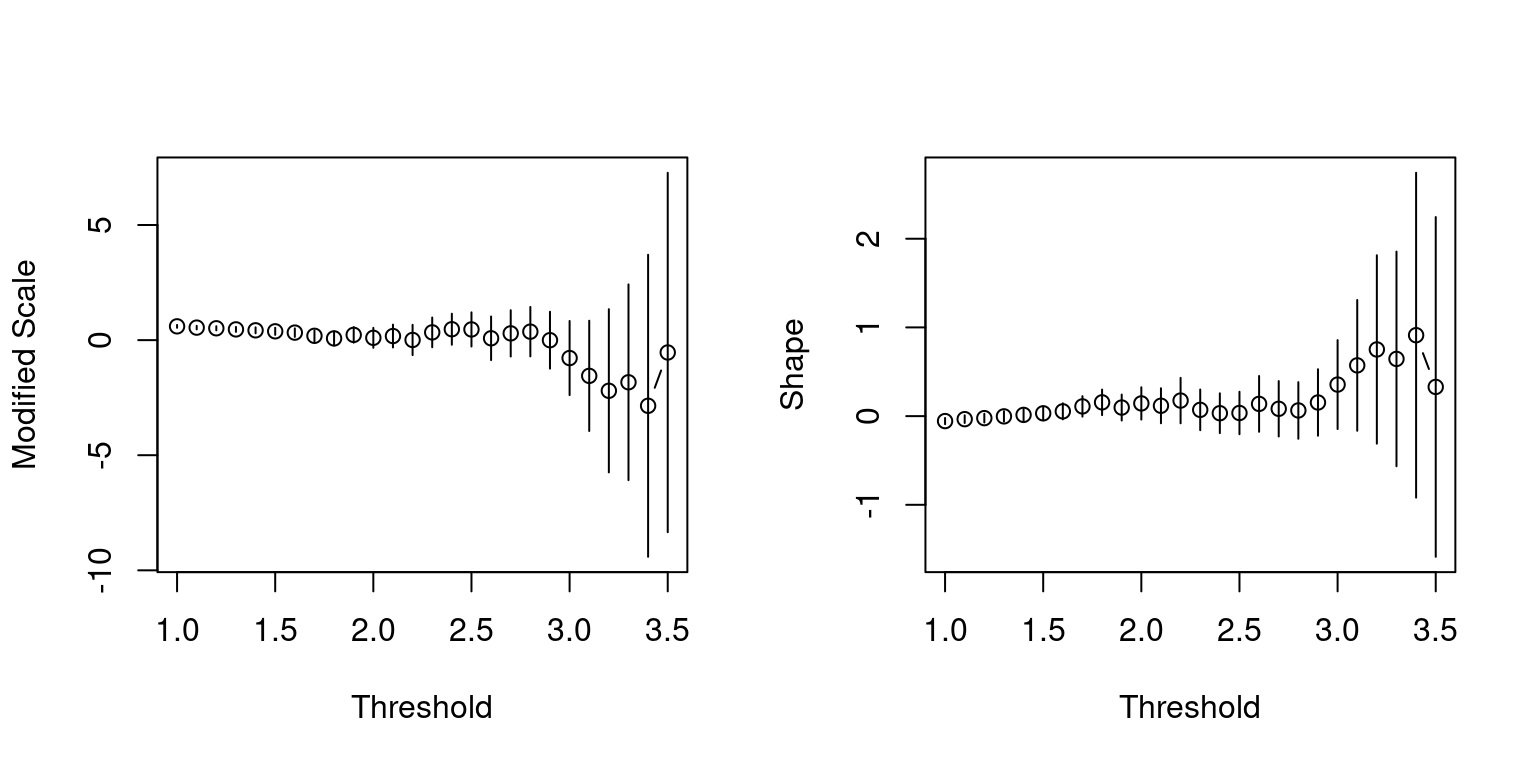
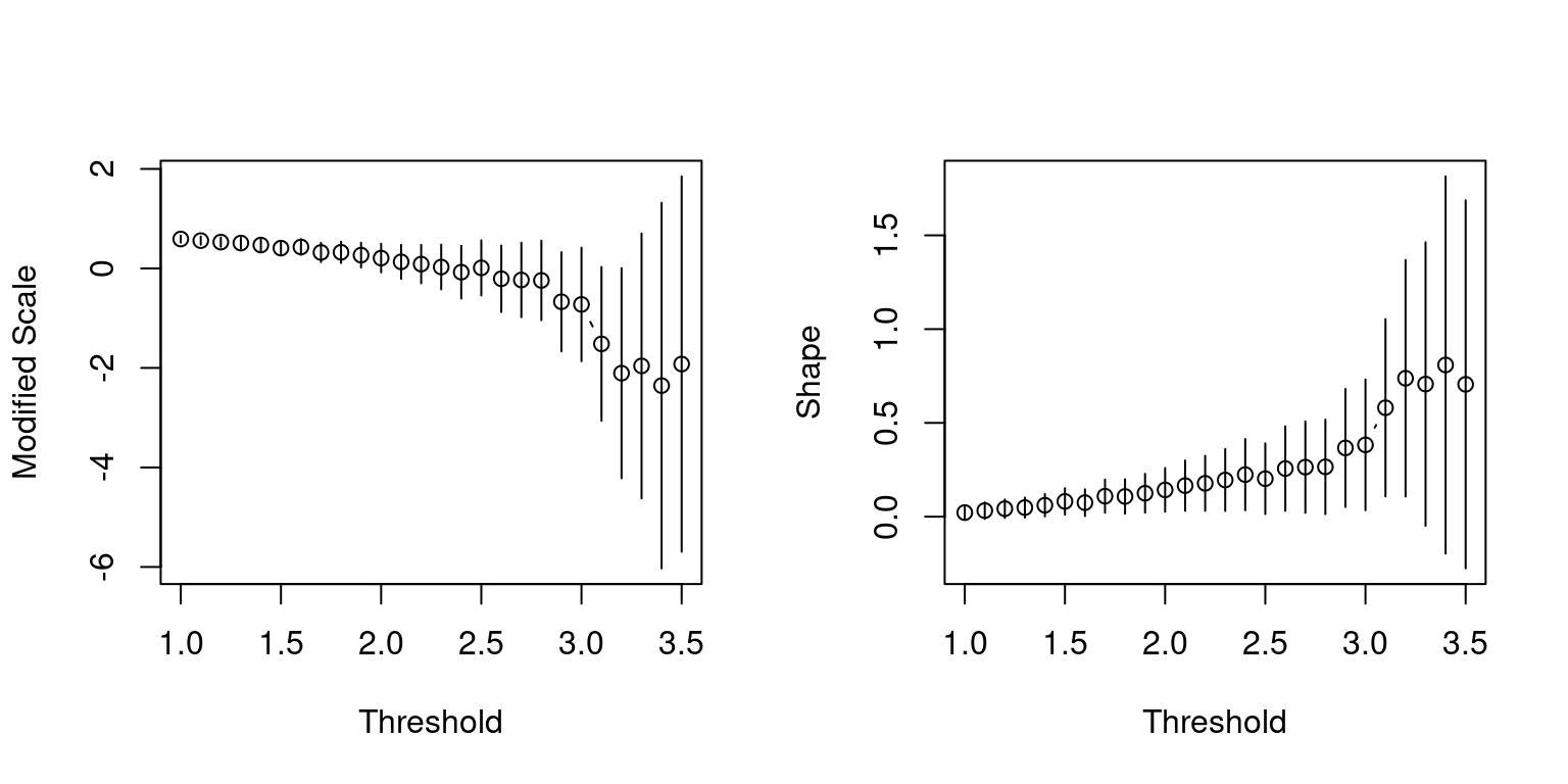
We can also fit the GPD to high quantiles to the residuals and the negative residuals to examine the behaviour on both tails. According to the parameter stability plots, it could be argued that the residuals (top) have a shape parameter of 0 i.e. the Gumbel distribution, whose DoA contains the normal distribution. On the other hand, it is quite clear that the negative residuals (bottom) have a heavier tail than what would be according to the normal distribution.
Ideally, the asymmetry and heaviness of the tails should be incorporated into the GARCH model. As such a unifying model is beyond the scope of this module, we will simply list out a few practical difficulties:
- Not even the Student’s \(t\)-distribution can circumvent the issue with the violation of the normality assumption, because the data are asymmetric in the tails, while the distribution itself is symmetric;
- Inherently, it is inconsistent to fit the GARCH model assuming normality first, followed by fitting non-normal distribution(s);
- If we are to fit the GARCH model while assuming the appropriate innovation distribution, we will need a distribution that encompasses not only the two tails but also the body;
- The two constraints of zero mean & unit variance for the innovations are still required.
See So and Chan (2014) for an example of incorporating extreme value methods in GARCH models.
7.5 Further reading
What is described in the section above is from a methodological point of view. For more theoretical results on the extremes of volatility models, please see de Haan et al. (1989), Breidt and Davis (1998), Mikosch and Stărică (2000), and Laurini and Tawn (2012). For some more examples of financial applications, see Figueiredo, Gomes, and Henriques-Rodrigues (2017) and Castro-Camilo, de Carvalho, and Wadsworth (2018).
Bibliography
Breidt, J. F., and R. A. Davis. 1998. “Extremes of Stochastic Volatility Models.” Annals of Applied Probability 8: 664–75.
Castro-Camilo, Daniela, Miguel de Carvalho, and Jennifer Wadsworth. 2018. “Time-Varying Extreme Value Dependence with Application to Leading European Stock Markets.” Annals of Applied Statistics 12 (1): 283–309. https://doi.org/10.1214/17-AOAS1089.
Coles, S. G., J. E. Heffernan, and J. A. Tawn. 1999. “Dependence Measures for Extreme Value Analyses.” Extremes 2: 339–65.
Coles, S. 1991. “Modelling Extreme Multivariate Events.” Journal of the Royal Statistical Society B 53: 377–92.
de Haan, L., S. I. Resnick, H. Rootzén, and C. G. de Vries. 1989. “Extremal Behaviour of Solutions to a Stochastic Difference Equation with Applications to ARCH Processes.” Stochastic Processes and Their Applications 32: 213–24.
Figueiredo, Fernanda, M. Ivette Gomes, and Lígia Henriques-Rodrigues. 2017. “Value-at-Risk Estimation and the PORT Mean-of-Order-P Methodology.” REVSTAT – Statistical Journal 15 (2): 187–204. https://ine.pt/revstat/pdf/rs170202.pdf.
Heffernan, J. E. 2000. “A Directory of Coefficients of Tail Dependence.” Extremes 3: 279–90.
Heffernan, J. 2004. “A Conditional Approach for Multivariate Extreme Values (with Discussion).” Journal of the Royal Statistical Society B 66 (3): 497–546.
Joe, H. 1997. Multivariate Models and Dependence Concepts. London: Chapman; Hall.
Laurini, F., and J. A. Tawn. 2012. “The Extremal Index for the GARCH\((1,1)\) Process.” Extremes 15: 511–29. https://doi.org/10.1007/s10687-012-0148-z.
Ledford, A. W., and J. A. Tawn. 1996. “Statistics for Near Independence in Multivariate Extreme Values.” Biometrika 83: 169–87.
Ledford, A. 1997. “Modelling Dependence Within Joint Tail Regions.” Journal of the Royal Statistical Society B 59: 475–99.
Ledford, A. 1998. “Concomitant Tail Behaviour for Extremes.” Advances in Applied Probability 30: 197–215.
Mardia, K. V. 1964. “Asymptotic Independence of Bivariate Extremes.” Calcutta Statistical Association Bulletin 13: 172–78.
Mikosch, T., and C. Stărică. 2000. “Limit Theory for the Sample Autocorrelations and Extremes of a GARCH\((1,1)\) Process.” Annals of Statistics 28: 1427–51.
Pickands, J. 1981. “Multivariate Extreme Value Distributions.” In Proceedings 43th, Session of International Statistical Institution, 859–78.
Sibuya, M. 1960. “Bivariate Extreme Statistics.” Annals of the Institute of Statistical Mathematics 11: 195–210.
So, M. K. P., and R. K. S. Chan. 2014. “Bayesian Analysis of Tail Asymmetry Based on a Threshold Extreme Value Model.” Computational Statistics and Data Analysis 71: 568–87.
Tiago de Oliveira, J. n.d. “Structure Theory of Bivariate Extremes; Extensions.” Est. Mat., Estat. E. Econ. 7: 165–95.
A slowly varying function satisfies \(\lim_{t\to\infty}L(tx)/L(t) = 1\), for any \(x>0\). Simple examples are \(L(x) = \log x\), and \(L(x) = C>0\), a positive constant.↩